plot: timeseries detrend

import numpy as np
import xarray as xr
import pandas as pd
import matplotlib.pyplot as plt
from datetime import timedelta, datetime
from geocat.viz import util as gvutil
import matplotlib.ticker as plticker
import matplotlib.dates as mdates
import cartopy.crs as ccrs
import cartopy.feature as cfeature
from geocat.viz import cmaps as gvcmaps

def detrend_polyfit(var, dim):
    #usage: det_sst = detrend_polyfit(sst_annmean,'year')
    p=var.polyfit(dim=dim, deg=1)
    fit = xr.polyval(var[dim], p.polyfit_coefficients)
    return var - fit

def detrend_theilsen(var, dim):
    #usage: det_sst = detrend_theilsen(sst_annmean.year.values, sst_annmean.values)
    from sklearn.linear_model import TheilSenRegressor
    
    x = var[dim].values
    y = var.values
    X = x[:,np.newaxis]
    reg = TheilSenRegressor(random_state=0).fit(X, y)
    score = reg.score(X, y)
    detrend = y - reg.predict(X)
    return xr.DataArray(detrend, dims=var.dims, coords=var.coords)

Reference figures

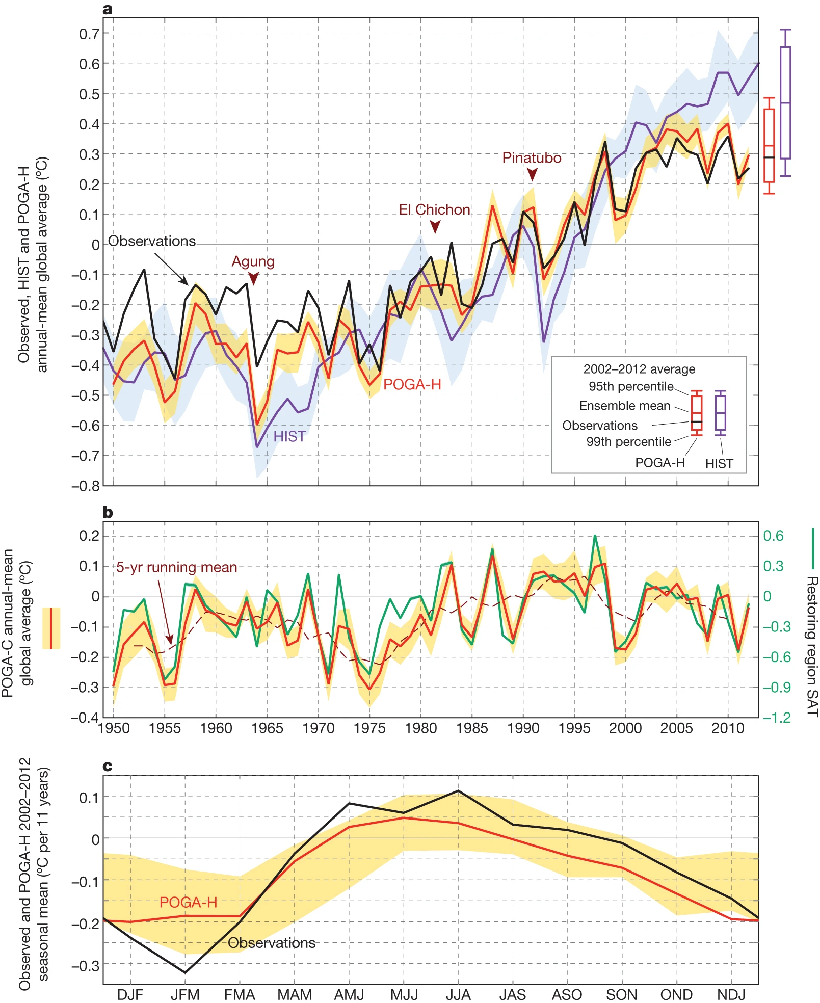
Fig. 1. Annual-mean time series based on observations, HIST and POGA-H (a) and on POGA-C (b). Anomalies are deviations from the 1980–1999 averages, except for HIST, for which the reference is the 1980–1999 average of POGA-H. SAT anomalies over the restoring region are plotted in b, with the axis on the right. Major volcanic eruptions are indicated in a. c, Trends of seasonal global temperature for 2002–2012 in observations and POGA-H. Shading represents 95% confidence interval of ensemble means. Bars on the right of a show the ranges of ensemble spreads of the 2002–2012 averages, from Kosaka and Xie (2013).

Read SST data

Read ERSSTv5

#date_range = pd.date_range('1950-01-01 00:00:00', '2012-12-31', freq='1M')
ds = xr.open_dataset('ERSSTv5_sst.mnmean.nc')
ersst = ds.sst.sel(time=slice('1850-01-01', '2021-12-31'))

sst_mnmean = ersst.weighted(weights = np.cos(np.deg2rad(ersst.lat))).mean(("lon", "lat"))
sst_annmean = sst_mnmean.groupby('time.year').mean('time')
sst_annmean = sst_annmean - sst_annmean.sel(year=slice(1961,1991)).mean('year')
ersst_detrend = detrend_theilsen(sst_annmean, dim='year')#.rolling(year=5, center=True).mean()
ersst_detrend

<xarray.DataArray (year: 168)>
array([ 0.22453785,  0.23995065,  0.12582968,  0.06818912,  0.11604401,
        0.22007604,  0.12877078,  0.06169266,  0.03209966,  0.12348787,
        0.16122619,  0.22388592,  0.23340311,  0.13953437,  0.16477001,
        0.16427171,  0.1407765 ,  0.15015827,  0.10735688,  0.06539663,
        0.00162013,  0.11122925,  0.04561406,  0.35148554,  0.29744605,
        0.14747647,  0.08508852,  0.13042571,  0.11827351,  0.0503695 ,
       -0.02506853, -0.08268048, -0.08309104, -0.11348131,  0.05757495,
        0.0601532 , -0.17748576, -0.03241712, -0.0889457 , -0.14009746,
       -0.16562208, -0.05550943,  0.06659473,  0.01423181, -0.14640749,
       -0.08864392, -0.00908126, -0.11586466, -0.19497434, -0.33271591,
       -0.4184479 , -0.22110647, -0.20975441, -0.27668376, -0.41083952,
       -0.45080278, -0.43241451, -0.42302893, -0.28926325, -0.33942509,
       -0.20116569, -0.13705446, -0.3091779 , -0.36483482, -0.23410945,
       -0.27519041, -0.27473694, -0.25311191, -0.30788382, -0.30957231,
       -0.31708012, -0.28329192, -0.1953293 , -0.25938237, -0.30526222,
       -0.35838808, -0.23668637, -0.20705429, -0.29072634, -0.33533399,
       -0.28459328, -0.29301662, -0.25837965, -0.17199059, -0.24837849,
       -0.18268225, -0.00614046,  0.12001873, -0.06594825, -0.09168078,
        0.06956599,  0.04669258, -0.21324137, -0.25016431, -0.2948349 ,
       -0.2646783 , -0.27407057, -0.19668992, -0.13626369, -0.14338813,
       -0.30503068, -0.33383213, -0.29447829, -0.11219347, -0.10131253,
       -0.16023483, -0.16570178, -0.14876501, -0.17052834, -0.16087001,
       -0.31881422, -0.28407044, -0.2355022 , -0.25478598, -0.24570749,
       -0.08890103, -0.1964302 , -0.32746172, -0.15061093, -0.13163902,
       -0.28810885, -0.30179456, -0.25814728, -0.10294299, -0.16725927,
       -0.04897744, -0.03860386, -0.07868537, -0.08283815, -0.01004277,
       -0.10902129, -0.15349924, -0.12467587,  0.01681839, -0.02773013,
       -0.07154813,  0.0229338 , -0.01536052, -0.09897726, -0.09667748,
       -0.07915897, -0.03973456, -0.08923646,  0.05507496,  0.09958436,
       -0.10552286, -0.08143544,  0.02837014,  0.05863927,  0.08179019,
        0.07015106,  0.06461163,  0.06196756, -0.01520806, -0.03413707,
        0.0862047 ,  0.09219519, -0.01760754,  0.04498734,  0.06306662,
        0.15073169,  0.26502716,  0.29920637,  0.2347909 ,  0.18676147,
        0.25817975,  0.23752077,  0.13383682])
Coordinates:
  * year     (year) int64 1854 1855 1856 1857 1858 ... 2017 2018 2019 2020 2021

Read HadCRUTv5

ds = xr.open_dataset('HadCRUT.5.0.1.0.analysis.anomalies.ensemble_mean.nc')
ds = ds.rename({"longitude":"lon", "latitude":"lat"})
ds.coords['lon'] = np.where(ds.coords['lon']<0, ds.coords['lon']+360, ds.coords['lon'])
ds = ds.sortby(ds.lon)

hadcrut = ds.tas_mean.sel(time=slice('1850-01-01', '2022-12-31'))
annmean = hadcrut.groupby('time.year').mean('time')

# global mean
gl_annmean = annmean.weighted(weights=np.cos(np.deg2rad(annmean.lat))).mean(("lon", "lat"))
gl_detrend = detrend_theilsen(gl_annmean, dim='year')

# Pacific Ocean mean
po = annmean.sel(lon=slice(130,280), lat=slice(-30,30))
po = po.weighted(weights=np.cos(np.deg2rad(po.lat))).mean(("lon", "lat"))
po_detrend = detrend_theilsen(po, dim='year')

# Indian Ocean mean
io = annmean.sel(lon=slice(40,120), lat=slice(-30,30))
io = io.weighted(weights=np.cos(np.deg2rad(io.lat))).mean(("lon", "lat"))
io_detrend = detrend_theilsen(io, dim='year')

# Maritime Continent
mc = annmean.sel(lon=slice(120,130), lat=slice(-30,30))
mc = mc.weighted(weights=np.cos(np.deg2rad(mc.lat))).mean(("lon", "lat"))
mc_detrend = detrend_theilsen(mc, dim='year')

#po_annmean.isel(year=100).plot()

Plot time-series of mean surface tempreature anomalies

fig, ax = plt.subplots(1,1, figsize=(9,4), constrained_layout=True, sharey=False)

year_slice = slice(1950, 2021)
gl_detrend = gl_detrend.sel(year=year_slice)
po_detrend = po_detrend.sel(year=year_slice)
io_detrend = io_detrend.sel(year=year_slice)
mc_detrend = mc_detrend.sel(year=year_slice)
gl_ersst_detrend = ersst_detrend.sel(year=year_slice)

lw = 1.5

x = gl_detrend.year
ax.plot(x, po_detrend, color='seagreen', lw=lw, ls='-', label='Pacific Ocean')
ax.plot(x, io_detrend, color='orangered', lw=lw, ls='-', label='Indian Ocean')
ax.plot(x, gl_detrend, color='k', lw=lw, ls='-', label='Global average')
#ax.plot(x, mc_detrend, color='royalblue', lw=lw, ls='-', label='Martime Continent')
ax.plot(x, gl_detrend.rolling(year=5, center=True).mean(), 
        marker='o', ms=6, mew=1, mfc='w', mec='k',
        color='k', ls='-', lw=3, label='Global average (5y moving)')
ax.plot(x, gl_ersst_detrend, color='k', lw=lw, ls=':', label='Global average_ERSSTv5')

ax.set_xticks(np.arange(1950,2025,5))
ax.axhline(0, c='k', lw=1, zorder=0)
ax.axvline(1998, c='lime', lw=1, zorder=0)

ax.axvline(1998, c='lime', lw=1, zorder=0)
ax.axvspan(1950, 1972, alpha=0.5, color='lightgrey', zorder=0)
ax.axvspan(2001, 2014, alpha=0.5, color='lightgrey', zorder=0)
ax.axvspan(2017, 2021, alpha=0.5, color='lightgrey', zorder=0)

ax.grid(True, ls=':', c='lightgray')
ax.legend(loc='upper left', prop=dict(size=12), frameon=False)

ax.set_title('detrended temperature anomalies from HadCRUT5', fontsize=18)
ax.set_xlabel('Year', fontsize=14)
ax.tick_params(axis='both', which='major', labelsize=12)
ax.set_ylabel('[degC]', fontsize=14)
ax.text(0.99, 0.01, "*relative to 1961-1990 reference period", 
        ha='right', va='bottom', fontsize=14, transform=ax.transAxes)

plt.show()
#sst_annmean_detrend

• Big hiatus: 1950-1972
• Slowdown of global warming or hiatus: 2001-2014
• large El Nino and La Nina events: 1998 and 2000
• 최근 5년은 뭐냐?

Read climate indices

ENSO (ONI)

### IPO (TPI)

PDO index

IOD

modes of climate variability (AO, AMO, …)

Read ERA5 data

ds = xr.open_dataset('ERA5_sst.mnmean_1deg.nc')
sst = ds.sst.sel(time=slice('1950-01-01', '2021-12-31'))

sst_mnmean = sst.weighted(weights = np.cos(np.deg2rad(sst.lat))).mean(("lon", "lat"))
sst_annmean = sst_mnmean.groupby('time.year').mean('time')
sst_annmean = sst_annmean - sst_annmean.sel(year=slice(1961,1991)).mean('year')
sst_annmean.plot()

[<matplotlib.lines.Line2D at 0x7f51aae83fd0>]

Read OISSTv2

# land-sea masking
#lsmask = xr.open_dataset("/mnt/e/OISSTv2/lsmask.oisst.v2.nc")['lsmask'].squeeze()

#date_range = pd.date_range('2016-07-01 00:00:00', '2016-09-06 00:00:00', freq='1D')
date_range = pd.date_range('2018-07-01 00:00:00', '2018-09-06 00:00:00', freq='1D')
year = date_range[0].strftime("%Y")

# Read OISSTv2 datasets.
mean = xr.open_dataset("sst.day.mean.{:}.nc".format(year))['sst']
err = xr.open_dataset("sst.day.err.{:}.nc".format(year))['err']
clim = xr.open_dataset("sst.day.mean.ltm.1991-2020.nc")['sst']

# Set a period range for this study and extract it from the Dataset.
mean = mean.sel(time=date_range)
err = err.sel(time=date_range)
clim = clim.isel(time=mean.time.dt.dayofyear.values-1)

# Extract regional basin around Korean Peninsula
minLon, maxLon, minLat, maxLat = [123, 129, 32, 39]
lon_slice, lat_slice = slice(minLon, maxLon), slice(minLat, maxLat)
mean = mean.sel(lon=lon_slice, lat=lat_slice)
err = err.sel(lon=lon_slice, lat=lat_slice)
clim = clim.sel(lon=lon_slice, lat=lat_slice)
clim['time'] = mean['time']

# If the error is greater than 0.2, drop it.
crit_err = 0.2
mean = mean.where(err<crit_err)
clim = clim.where(err<crit_err)

# Create a latitude weight and apply it to all variables.
weights = np.cos(np.deg2rad(mean.lat))
weights.name = "weights"
weighted_mean = mean.weighted(weights).mean(("lon","lat"))
weighted_clim = clim.weighted(weights).mean(("lon","lat"))

#err.sel(time="2016-08-15")

/home/siyang/miniconda3/envs/jupyter/lib/python3.8/site-packages/xarray/coding/times.py:527: SerializationWarning: Unable to decode time axis into full numpy.datetime64 objects, continuing using cftime.datetime objects instead, reason: dates out of range
  dtype = _decode_cf_datetime_dtype(data, units, calendar, self.use_cftime)
/home/siyang/miniconda3/envs/jupyter/lib/python3.8/site-packages/numpy/core/_asarray.py:83: SerializationWarning: Unable to decode time axis into full numpy.datetime64 objects, continuing using cftime.datetime objects instead, reason: dates out of range
  return array(a, dtype, copy=False, order=order)

Visualization

fig, ax = plt.subplots(1,1, subplot_kw=dict(projection=ccrs.PlateCarree()))

ax.coastlines(linewidths=0.5)
ax.add_feature(cfeature.LAND, facecolor='lightgray')
mesh = ax.pcolormesh(err.lon, err.lat, err.sel(time="2016-08-15").values, cmap=gvcmaps.MPL_jet)
cbar = fig.colorbar(mesh)
cs = ax.contour(err.lon, err.lat, err.sel(time="2016-08-15"), colors='w', linewidths=[5], levels=[0.2])
gvutil.set_axes_limits_and_ticks(ax,xlim=(minLon, maxLon), ylim=(minLat, maxLat),
                                 xticks=np.arange(120, 130, 2),
                                 yticks=np.arange(30, 42, 2))
gvutil.add_lat_lon_ticklabels(ax)

ax.coastlines(linewidths=0.5, zorder=101)
ax.add_feature(cfeature.LAND, facecolor='lightgray', zorder=100)

#plt.show()
fig.savefig('fig_OISSTv2_dist_err_20180810.png', dpi=500, bbox_inches='tight')

/home/siyang/miniconda3/envs/wrf_tutorial/lib/python3.8/site-packages/cartopy/mpl/geoaxes.py:1491: MatplotlibDeprecationWarning: shading='flat' when X and Y have the same dimensions as C is deprecated since 3.3.  Either specify the corners of the quadrilaterals with X and Y, or pass shading='auto', 'nearest' or 'gouraud', or set rcParams['pcolor.shading'].  This will become an error two minor releases later.
  X, Y, C = self._pcolorargs('pcolormesh', *args, allmatch=allmatch)



---------------------------------------------------------------------------

ValueError                                Traceback (most recent call last)

/tmp/ipykernel_253/3744171931.py in <module>
      3 ax.coastlines(linewidths=0.5)
      4 ax.add_feature(cfeature.LAND, facecolor='lightgray')
----> 5 mesh = ax.pcolormesh(err.lon, err.lat, err.sel(time="2016-08-15").values, cmap=gvcmaps.MPL_jet)
      6 cbar = fig.colorbar(mesh)
      7 cs = ax.contour(err.lon, err.lat, err.sel(time="2016-08-15"), colors='w', linewidths=[5], levels=[0.2])


~/miniconda3/envs/wrf_tutorial/lib/python3.8/site-packages/cartopy/mpl/geoaxes.py in pcolormesh(self, *args, **kwargs)
   1457                              ' consider using PlateCarree/RotatedPole.')
   1458         kwargs.setdefault('transform', t)
-> 1459         result = self._pcolormesh_patched(*args, **kwargs)
   1460         self.autoscale_view()
   1461         return result


~/miniconda3/envs/wrf_tutorial/lib/python3.8/site-packages/cartopy/mpl/geoaxes.py in _pcolormesh_patched(self, *args, **kwargs)
   1489         allmatch = (shading == 'gouraud')
   1490 
-> 1491         X, Y, C = self._pcolorargs('pcolormesh', *args, allmatch=allmatch)
   1492         Ny, Nx = X.shape
   1493 


ValueError: too many values to unpack (expected 3)


/home/siyang/miniconda3/envs/wrf_tutorial/lib/python3.8/site-packages/cartopy/mpl/geoaxes.py:387: MatplotlibDeprecationWarning: 
The 'inframe' parameter of draw() was deprecated in Matplotlib 3.3 and will be removed two minor releases later. Use Axes.redraw_in_frame() instead. If any parameter follows 'inframe', they should be passed as keyword, not positionally.
  return matplotlib.axes.Axes.draw(self, renderer=renderer,

fig, ax = plt.subplots(1,1, subplot_kw=dict(projection=ccrs.PlateCarree()))

cmap = gvcmaps.MPL_jet.copy()
cmap.set_bad("k")
mesh = ax.pcolormesh(mean.lon, mean.lat, mean.sel(time="2016-08-15"), cmap=cmap, zorder=1)
cbar = fig.colorbar(mesh)
gvutil.set_axes_limits_and_ticks(ax,xlim=(minLon, maxLon), ylim=(minLat, maxLat),
                                 xticks=np.arange(120, 130, 2),
                                 yticks=np.arange(30, 42, 2))
gvutil.add_lat_lon_ticklabels(ax)

ax.coastlines(linewidths=0.5, zorder=101)
ax.add_feature(cfeature.LAND, facecolor='lightgray', zorder=100)

#plt.show()
fig.savefig('fig_OISSTv2_dist_mean_20180810.png', dpi=500, bbox_inches='tight')

/home/siyang/miniconda3/envs/wrf_tutorial/lib/python3.8/site-packages/cartopy/mpl/geoaxes.py:1491: MatplotlibDeprecationWarning: shading='flat' when X and Y have the same dimensions as C is deprecated since 3.3.  Either specify the corners of the quadrilaterals with X and Y, or pass shading='auto', 'nearest' or 'gouraud', or set rcParams['pcolor.shading'].  This will become an error two minor releases later.
  X, Y, C = self._pcolorargs('pcolormesh', *args, allmatch=allmatch)



---------------------------------------------------------------------------

ValueError                                Traceback (most recent call last)

/tmp/ipykernel_253/2448314526.py in <module>
      3 cmap = gvcmaps.MPL_jet.copy()
      4 cmap.set_bad("k")
----> 5 mesh = ax.pcolormesh(mean.lon, mean.lat, mean.sel(time="2016-08-15"), cmap=cmap, zorder=1)
      6 cbar = fig.colorbar(mesh)
      7 gvutil.set_axes_limits_and_ticks(ax,xlim=(minLon, maxLon), ylim=(minLat, maxLat),


~/miniconda3/envs/wrf_tutorial/lib/python3.8/site-packages/cartopy/mpl/geoaxes.py in pcolormesh(self, *args, **kwargs)
   1457                              ' consider using PlateCarree/RotatedPole.')
   1458         kwargs.setdefault('transform', t)
-> 1459         result = self._pcolormesh_patched(*args, **kwargs)
   1460         self.autoscale_view()
   1461         return result


~/miniconda3/envs/wrf_tutorial/lib/python3.8/site-packages/cartopy/mpl/geoaxes.py in _pcolormesh_patched(self, *args, **kwargs)
   1489         allmatch = (shading == 'gouraud')
   1490 
-> 1491         X, Y, C = self._pcolorargs('pcolormesh', *args, allmatch=allmatch)
   1492         Ny, Nx = X.shape
   1493 


ValueError: too many values to unpack (expected 3)


/home/siyang/miniconda3/envs/wrf_tutorial/lib/python3.8/site-packages/cartopy/mpl/geoaxes.py:387: MatplotlibDeprecationWarning: 
The 'inframe' parameter of draw() was deprecated in Matplotlib 3.3 and will be removed two minor releases later. Use Axes.redraw_in_frame() instead. If any parameter follows 'inframe', they should be passed as keyword, not positionally.
  return matplotlib.axes.Axes.draw(self, renderer=renderer,

fig, ax = plt.subplots(1,1, figsize=(8,3))

loc = plticker.MultipleLocator(base=7)

ax.plot(mean.time, weighted_clim, lw=3, color='k', label='climatology')
ax.plot(mean.time, weighted_mean, lw=1.5, color='k', label='daily average', ls=':')

ax.fill_between(mean.time, weighted_mean, weighted_clim, 
                where=(weighted_mean > weighted_clim), 
                color='orangered', alpha=0.8, interpolate=True)
ax.fill_between(mean.time, weighted_mean, weighted_clim, 
                where=(weighted_mean < weighted_clim), 
                color='dodgerblue', alpha=0.8, interpolate=True)

date0 = datetime(2018, 8, 15, 0, 0)
date1 = date0 + timedelta(days=0)
date2 = date1 + timedelta(days=10)
print(" *spin-up (week):     ", date0, '~', date1)
print(" *simulation (month): ", date1, '~', date2)
for d in [date0, date1, date2]:
    ax.axvline(d, color='k', c='orange', lw=2)
    
ax.set_yticks(np.arange(21,30,1))
ax.spines['top'].set_visible(False)
#ax.set_title('Time series for weighted mean SST', fontsize=18)
ax.set_ylabel('[degC]', fontsize=13)
ax.set_xlabel('Date', fontsize=13)
ax.tick_params(axis='x', labelsize=10)
ax.tick_params(axis='y', labelsize=10)
ax.axhline(28, color='grey',  lw=1, ls='--')

ax.xaxis.set_major_locator(loc)
ax.xaxis.set_major_formatter(mdates.DateFormatter('%d\n%b'))

ax.legend(loc='best', prop=dict(size=9), frameon=False)
fig.savefig('fig_OISSTv2_ts_mean_2018.png', dpi=500, bbox_inches='tight')

 *spin-up (week):      2018-08-15 00:00:00 ~ 2018-08-15 00:00:00
 *simulation (month):  2018-08-15 00:00:00 ~ 2018-08-25 00:00:00

fig, ax = plt.subplots(1,1, figsize=(8,3))

loc = plticker.MultipleLocator(base=7)

date0 = datetime(2018, 7, 15, 0, 0)
date1 = date0 + timedelta(days=7)
date2 = date1 + timedelta(days=31)

print(" *spin-up (week):     ", date0, '~', date1)
print(" *simulation (month): ", date1, '~', date2)

for d in [date0, date1, date2]:
    ax.axvline(d, color='k', c='orange', lw=2)

ax.plot(mean.time, weighted_anom, lw=1.5, ls='-', color='k')
ax.fill_between(mean.time, weighted_anom, where=(weighted_anom > 0), color='red', alpha=0.3, interpolate=True)
ax.fill_between(mean.time, weighted_anom, where=(weighted_anom < 0), color='blue', alpha=0.3, interpolate=True)
ax.set_yticks(np.linspace(-1,3,5))  
ax.axhline(0, color='k', lw=1)
ax.spines['top'].set_visible(False)
ax.tick_params(axis='x', labelsize=10)
ax.tick_params(axis='y', labelsize=10)
ax.set_ylabel('[degC]', fontsize=13)
ax.set_xlabel('Date', fontsize=13)

ax.xaxis.set_major_locator(loc)
ax.xaxis.set_major_formatter(mdates.DateFormatter('%d\n%b'))

fig.savefig('fig_OISSTv2_ts_anom.png', dpi=500, bbox_inches='tight')

 *spin-up (week):      2018-07-15 00:00:00 ~ 2018-07-22 00:00:00
 *simulation (month):  2018-07-22 00:00:00 ~ 2018-08-22 00:00:00